Read Part 1 of the Binance Blog Trader Series Here.
Key Takeaways
- The author analyzed how two trading systems, namely the trend hybrid system and the divergence system, performed against the typical buy-and-hold strategy for investing in cryptocurrencies.
- A trend-following strategy seemed the most appropriate to use in order to take advantage of bitcoin’s strong trends, but it also performed reasonably well on other altcoins without any further optimization, except for the stop loss ATR parameter to take into account the higher volatility of altcoins.
- The author devised a divergence strategy specifically for ETH, in order to exploit its lagging correlation with Bitcoin, but it also performed equally well or better on the other cryptocurrencies.
- The technical approach seems a reasonable way to trade cryptocurrencies because it blocks out a lot of the noise by only focusing on the price action and supporting technical and intermarket indicators
The views and opinions of Markos Katsanos do not necessarily reflect those of the Binance blog, Binance, or its divisions and affiliates. Please exercise due diligence when reading this.
Prelude to Trading Tips
Before divulging any strategies I should point out, for the benefit of traders that are not familiar with cryptocurrencies, that these are highly volatile assets, far more than the traditional stocks or forex that you are accustomed to trading. You should therefore revise trading rules, such as stops or profit targets based on percentages.
In the second part of this article, I will present two trading strategies for trading cryptocurrencies. Within a developed simulation environment algorithms, the cryptos are put to the test, and conclusions are drawn regarding both the prediction accuracy and the test procedure as such. The first is basically a trend following system, enhanced by adding Intermarket conditions. The second is mainly a divergence system that exploits the strong cross-correlation between cryptocurrencies.
Trend Hybrid System
A trend-following strategy seemed the most appropriate to use in order to take advantage of bitcoin’s strong trends.
After preliminary testing of some popular trend systems, I decided to use a simple Donchian breakout channel system. The channel is derived by calculating the Highest and Lowest prices for a pre-defined period. The autocorrelation analysis indicated that the autocorrelation of 30-day returns was very strong up to 15 days in the future so I based this strategy on the breakout of a 30-day Donchian channel. Any breakout of the upper or lower band triggered buy or short signals, respectively. I used an additional middle band by taking the mean of the upper and lower bands. This middle band was utilized to exit long or short positions.
Additionally, I introduced a Chandelier Trailing stop loss into the system for risk management. At first glance, the drawdown of the system was on the high side so in order to improve the accuracy of the entry signal I decided to add a long term (100-day period) moving average trend filter. Thus when the price is above the 100-period moving average, the system would only look for breakouts to the upside; and when the price is below the 100-period moving average, for short breakouts.
In the next step and in order to take advantage of the strong directional correlation between bitcoin and the S&P 500, I added an Intermarket filter which filtered out trades when the bitcoin broke out in the opposite direction of the S&P 500. The filters described above reduced trend trades considerably, so only one was deployed at any time, i.e., the channel breakout signal was executed if either of the filters was true. Trend following systems does not produce trades in sideways or choppy markets so
In order to increase the number of trades, I added a second condition mean reversion signal which exploited bitcoin’s relative value with gold. The final system can be summarized as follows:
A. Buy Conditions
Channel. A buy signal was generated if the price broke out above a 30-day channel but only if the price was above the 100-day moving average or the S&P 500 was in an uptrend. To determine the S&P 500 directional trend, I used its 30-day moving average. Daily high or Low prices varied considerably between exchanges so I used the closing price for breakouts.
Oversold. The effect of mean reversion is exploited in trading strategies and it involves ‘buying low’ and ‘selling high’. This effect refers to the waves of optimism and pessimism that give the market inertia to temporarily move asset prices away from their “real” value. To determine bitcoin’s real value I used bitcoin’s ratio with Gold to determine oversold or overbought levels (see figure 2 above) and refined the signals with the short term (10-day) stochastic oscillator. The BTC/Gold ratio was normalized from 0 (oversold) to 100 (Overbought) during the last 250 day period. To calculate this ratio I used the Gold ETF (GLD) but since the ratio is normalized, the absolute Gold price is irrelevant, so you can also use Gold cash prices or Gold futures.
A problem with using oscillators is that they are often too early to buy or sell in a trending market so I used the Congestion Index (CI), to filter out trades in trending markets. Thus trades were only considered when the 30-day CI was below 30. The CI is a custom trend indicator similar to Wilder’s ADX or the Vertical Horizontal filter, that I introduced in my book (see suggested reading).
B. Sell (Close Long) Conditions:
Long positions were closed if the price fell below the middle channel line.
I also used a Chandelier trailing stop loss based on a 10 Periods of Average True Range (ATR) which closed the trade if the price fell 2 ATR below the highest price of the last 2 days. All stops were executed the next day at the open. The best stop parameters were chosen by walk forward optimization.
Finally a 15 day time exit closed all trades if neither of the stops was activated.
To choose the trade duration I didn’t use optimization but selected the highest lag value from the autocorrelation table in figure 13 with reasonably strong lagging autocorrelation for 25-30 day returns.
C. Sell Short Conditions:
The short or buy to cover conditions were the exact opposite of the buy conditions described above and there was no long or short bias in the system.
In order to avoid the illusion of optimization or curve fitting, I didn’t optimize any of the parameters used for the channel length but selected the shortest time with the best autocorrelation which was about 30 days. For the moving average trend period, I chose the popular moving average period of 100 days. In order to avoid the pitfall of curve fitting, I used the walk forward optimization method to select the most robust parameters for the Chandelier stop loss, the stochastic period and overbought or oversold levels. Of course, nothing can guarantee future results, but this approach appears to be as close as we can practically come to estimating trading parameters during constantly changing market conditions.
To perform the walk forward optimization I divided all available data during the last 9 years since May 25, 2011, into five data sets, 18 months each. I then optimized the system using the first sub-period and tested it out of the sample using the next period. Once this test was completed, the whole time window was moved forward 18 months to include the period just tested and the system was then re-optimized. It was then tested again using the next data set. This process was repeated again and again, “walking forward” through the data series until I ran out of data. In the end, all tabulated one-year out-of-sample results were merged to create one large out-of-sample results segment and the system performance was evaluated based on the combined out-of-sample results.
To test the performance of the other altcoins I didn’t optimize any of the parameters except for the stop loss parameter. Altcoins are more volatile than bitcoin so increasing the stop-loss margin improved the performance on 3 out of five altcoins.
Test Procedure
A problem in backtesting the strategy was the variability of data between different crypto exchanges so for this simulation testing I decided to use Crypto Index data from Investing.com, which takes the average prices from all exchanges. The data used for these tests included weekends, therefore this system is not appropriate for trading bitcoin futures on the CME as they only trade on business days. If you want to use it to trade futures then you will have to adjust the ATR parameters in order to take into account the higher volatility on Mondays as well as all indicator periods and trade duration to take into account the shorter weekdays.
Another problem was the large price variation in bitcoin prices during the test duration resulting in hugely different trading amounts so I decided to specify a constant US dollar amount for the default trade size and one decimal point for the round lot size.
The initial capital was $22,000, the trade size $20,000, and the round lot 0.10 coins. The trade duration was eight years from May 28, 2012, to May 28, 2020, for bitcoin. The other altcoins started trading later so the testing period varied from 2.6 years for the BNB to 4.2 years for the ETH. Long and short signals were executed the next day at the open and no interest was credited to the account when out of the market as this was assumed to cancel out additional slippage and skid costs. The commission 0.1% was deducted from each trade. The system did not reinvest profits. The total return would obviously be far larger if the returns were compounded.
To evaluate the efficacy of the system, I compared its performance with the standard benchmark Buy & Hold strategy which involved buying and holding an equal dollar amount of bitcoins for the last three and eight-year test periods until the end of May 2018.
Evaluation
In the table, in Figure 16 below, you can see the test simulation results of a 3-year and 8-year backtest compared to the Buy & Hold for bitcoin and the performance of the same system on another five popular altcoins.
The comparison with the Buy & Hold strategy was not very pertinent because of Bitcoin’s meteoric 187,000 % surge from $5.10 at the beginning of the test to $9,572 at the end. This is impossible to beat on a net profit basis. Nevertheless, the system improved on the risk characteristics significantly, reducing the maximum drawdown significantly from a catastrophic 91% of equity or -$63 million to a manageable 16.5% or $16,000 for bitcoin.
A more realistic comparison between the system and the Buy & Hold is during the last 3-year period (see Figure 16, in the first two columns). In this case, the system managed to beat the benchmark on both net profit and risk basis.
The system produced most of the profits on the long side with the short trades contributing only 15% of the profits and adversely impairing drawdown and all other metrics.
This is because the bitcoin price was predominantly bullish during the test period as there was no long bias in the system. In the future, however, this may not be the case.
You might have noticed that the percentage of profitable trades for the XRP and BCH is only 45%. Keep in mind that you don’t need this to be greater than 50% for a profitable system if you make more on winning trades than you lose on losing trades. In order to determine the system profitability, you should use the percentage wins in conjunction with the Win/Loss ratio or payout. In this case, XRP profitable trades produced 6 times more profits then losing trades thus producing more profits than other altcoins with a higher percentage of winning trades.
In order to gain more insight into the risk characteristics and robustness of the system, I decided to analyze the system performance with the Monte Carlo method by performing random sampling of the actual trade list generated by the back-test and computing the system equity for each sample.
As you can see in the table in Figure 17 and graphically in Figure 18, the Monte Carlo simulation results were very encouraging. The probability of the maximum drawdown exceeding 31% was only 1% and the final equity was always profitable. As you can see in the charts in figure 18 there was a 25% chance that the minimum equity line (in red) will fall below the initial equity which will happen only if the majority of the unprofitable trades are rearranged at the start of the test.
Despite the fact that the Trend Hybrid system was developed and optimized for bitcoin it performed reasonably well on all other altcoins (see Figure 16) without any further optimization except for the stop loss ATR parameter to take into account the higher volatility of the altcoins (see figure 15). The best performer was the ETH on a profit factor and % profitable basis and the XRP on a net profit basis. Keep in mind that the maximum % drawdown statistic is not very indicative of the system’s risk as it depends on the equity value at the time of maximum drawdown. Thus if the drawdown occurred on low equity (usually in the beginning of the test) the drawdown % would be high. This is obvious in the case of ETH where the maximum drawdown in % terms was 53% of equity whereas in dollar terms it was only $16,400.
In the 3D optimization chart in Figure 19 you can see that the strategy was profitable for channel lengths (CL) from 25 to 40 days and holding periods (exit) from 10 to 20 days.
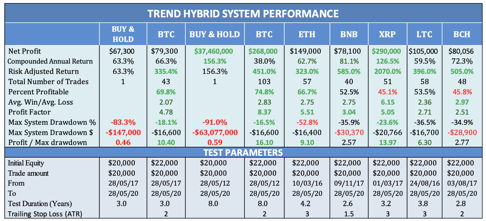
Figure 16. You can see here the system performance during the last 3 and 8 year period until May 28, 2020, for BTC. The other altcoins started trading later so the testing period varied according to the available data. The Risk-adjusted return (RAR) (third row) is the Net profit divided by Exposure and is calculated on a bar by bar basis. The single bar exposure is the value of open positions divided by portfolio equity. The Profit Factor is the ratio of gross winnings to gross losses. The Profit/ Max drawdown (last row) is calculated by dividing the Net profit by the max. system drawdown.
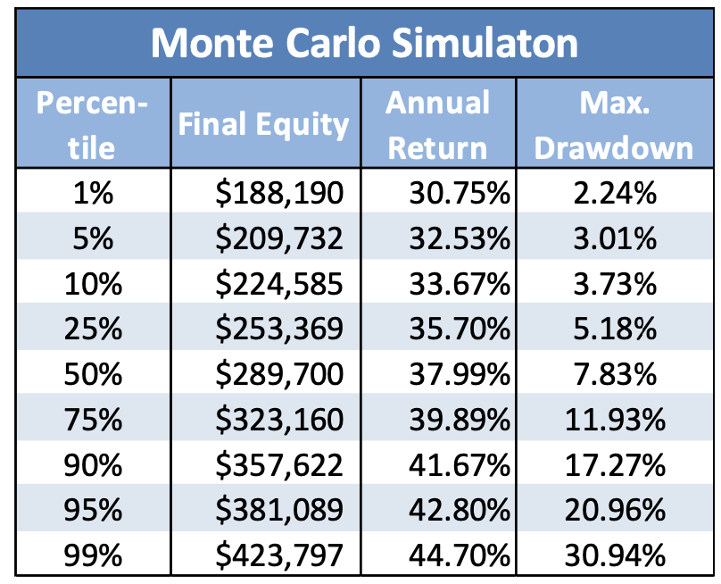
Figure 17. Key statistics derived from the cumulative distribution charts (CDFs) of Monte Carlo simulation results. Starting equity was $22000 and the test duration 8 years (EOD data). The first column shows the percentile level (the value below which a given percentage of test observations fall). So the 95th percentile tells us that 95% of the time observed value is below the shown amount. For example, the max drawdown at the 95th percentile (in this case 21%) means that 95% of tests had drawdowns of less than 21%. So we can say that there is a 5% chance that it will be higher than that. If we look further in the table we can also notice that in 99% of the cases, drawdowns will be less than 31%.
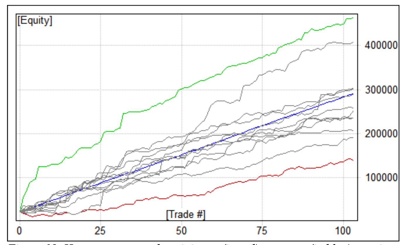
Figure 18. Here you can see the minimum (in red), average (in blue), maximum (green), and various in between straw broom charts of simulated Monte Carlo equities simulation results. Note that green and red lines (min/max equity) are not really single "best" and "worst" equities. They are bar-by-bar highest (max) and lowest (min) points of ALL equities generated during the Monte Carlo Simulation. The blue line (avg) is the average of all equity lines (all runs). The 'cloud' of gray lines represents individual test equities - as we can see the same trading system may generate different outcomes when market conditions change and MC simulation attempts to simulate various outcomes and provide you with some statistical information on how bad/good it may be. Starting equity was $22000 and the test duration 8 years.
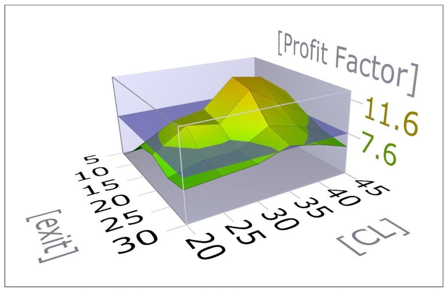
Figure 19. 3D chart of the bitcoin Trend Hybrid System parameters from May 2012 until the end of May 2020. The system was optimized for values of the channel period from 20 to 45 days on the X-axis and holding periods from 5 to 30 days on the y-axis. The Profit factor is plotted on the Z-axis. Parameter combinations producing a profit factor >7.5 protrude above the waterline (blue horizontal plane).
Divergence System
This system exploits the strong correlation between cryptocurrencies. To calculate the divergence between various currencies I used the Regression Divergence indicator presented in Chapter 9 of my book Intermarket Trading Strategies (see suggested reading). This indicator can be used to calculate the divergence between a security and a related market by regressing the rate of change between the two securities and then calculating the difference of the actual from the forecasted price. The divergence is then normalized on a scale from 0 to 100 and buy signals are generated when the indicator reaches a peak above a certain level (usually 75-80%) and subsequently declines. Similarly sell signals are triggered when the indicator reaches a bottom below a certain level (usually 25 to 20%) and rises. To find the best-correlated currencies and time interval for the rate of change I used the tables in figures 5, 6, and 7 and the leading/lagging analysis in figures 10 & 11.
My first choice was to design a system to trade Ether given its strong lagging correlation with bitcoin. To calculate the divergence I used daily returns since these had the strongest correlation (r=0.84 in figure 5) with the bitcoin.
Divergence systems do not usually produce a lot of signals so in order to increase the number of trades I added a second trend condition. This doubled the number of trades with about half the signals generated by divergence and the other half by the trend condition. To test the system I used crypto Index historical data from investing.com and the same test specifications with the Trend Hybrid system described above.
The final system can be summarized as follows:
Long Divergence Condition:
A buy signal was generated if the maximum divergence rose over 75 and then reversed direction during the next 6 days while at the same time the bitcoin was trending up during the preceding 3 day period.
Long Trend Signal:
For this condition, I used the 30 day channel breakout condition without any optimization. In this case, in order, in order to filter out trades during consolidating trendless markets I used correlation directly as an indicator by correlating prices with a straight line at a 45o angle.
Thus if the trend is up, the correlation with the straight line is positive, ranging from +0.70 to a maximum of +1.0. If the trend is down the correlation is negative, ranging from -0.70 to -1.0. If the price trend is sideways then there is no correlation over the correlation period span
In this case, long trend signals were filtered out if the correlation over the channel length was less than 0.70.
Short Divergence Condition:
The sell short divergence condition is the reverse of the buy condition described above Short signals were triggered if the divergence fell below 20 and reversed direction. Short Trend condition:
This is again the reverse of a long trend with no long or short bias in the system. Trend signals were filtered out if the correlation trend was more than -0.70.
Sell (Close Long) Conditions:
I used one sell condition to close divergence trades and one for trend trades. The divergence exit closed the trade if the normalized divergence fell below 20 and then started to rise while the raw divergence was below zero. The trend exit closed the trade if the correlation trend turned negative.
I also used the following trailing stop condition in case something went wrong: The trade was closed if the price fell 2.5 ATR below the highest price during the last four days. This was deployed only if the price was below its 20 day moving average.
If none of the above conditions were triggered than all positions were closed 15 calendar days (including weekends) at the latest.
All trades were executed the next day at the open.
Buy to cover Conditions. These were again the exact opposite of the sell conditions described above.
I used walk forward optimization to select the most robust parameters for the long and short divergence thresholds, the regression length, the critical correlation trend, the BTC % rate of change, and the trailing stop parameters for the ETH test. For the BTC and other altcoins, I didn’t optimize any parameters except for the trailing stop ATR parameter and the return period (ROC) used to calculate the divergence. This varied from 1 day for ETH and XRP, 2 days for BNB and LTC, and 3 days for the BTC test. The trailing stop ATR varied from 2 to 3.
For the other tests, I used correlation tables in order to select the cryptocurrency with the strongest correlation for the divergence calculation. All altcoins correlated best with the ETH, except for the BCH which preferred the LTC. For the BTC test, I used the next best altcoin (LTC) as the correlation with ETH was lagging. You can see the test parameters for all cryptocurrencies in Figure 20.
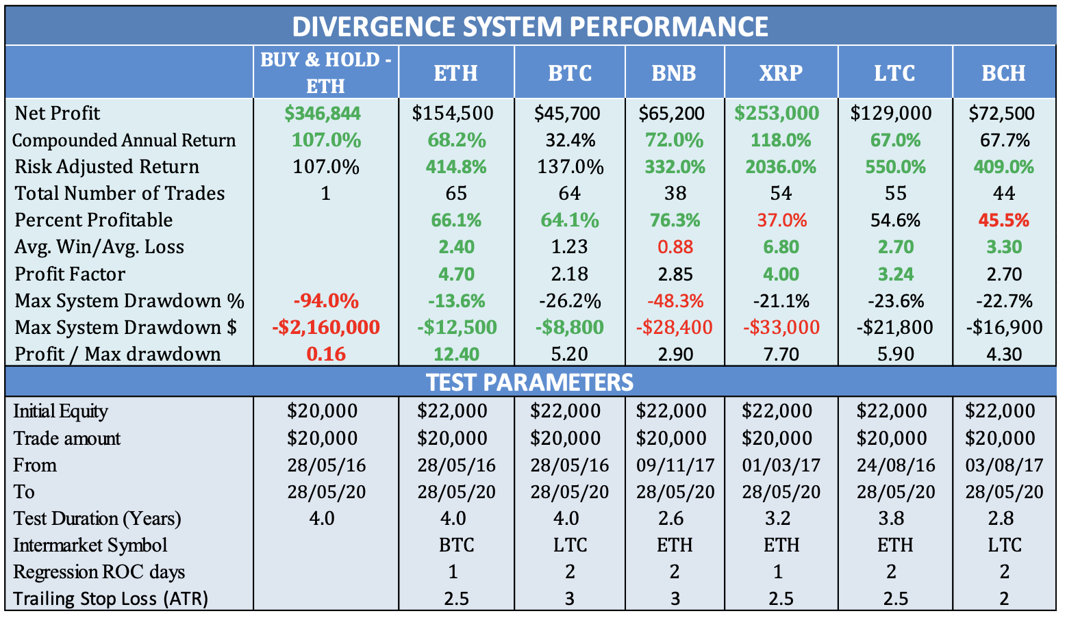
Figure 20. You can see here the system performance during the last 4 year period until the 28th of May 2020 for ETH and BTC. The other altcoins started trading later so the testing period varied according to the available data. For an explanation of the test statistics please see the legend in Figure 16 above. The test was designed and optimized for ETH only. Because of varying volatilities, I only optimized the ATR trailing stop parameter for the other cryptocurrency tests.
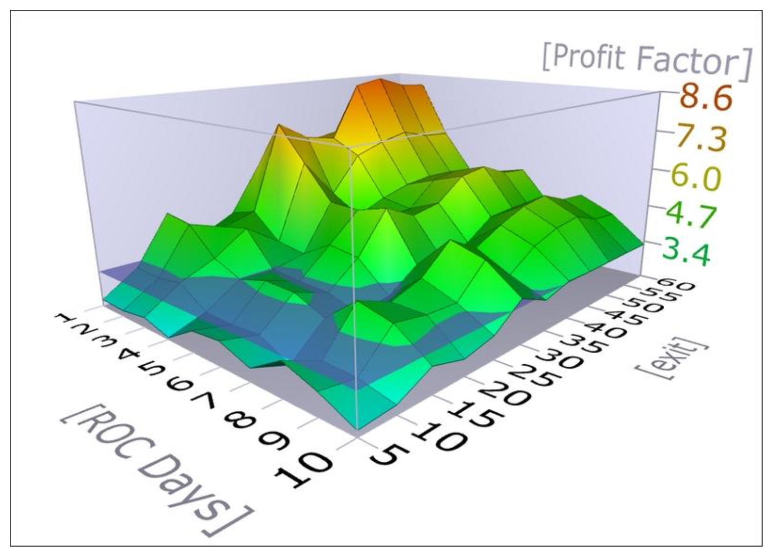
Figure 21. 3D chart of the ETH Divergence System parameters from May 28, 2016, until the end of May 2020. The system was optimized for values of the return ROC period (for the Regression divergence calculation) from 1 to 10 days on the Y-axis and holding periods from 5 to 60 days on the y-axis. The Profit factor is plotted on the Z-axis. Parameter combinations producing a profit factor >3 protrude above the waterline (blue horizontal plane).
Evaluation
In the table in Figure 20, you can see the test simulation results of a 4-year backtest compared to the Buy & Hold forETH
The comparison with the Buy & Hold strategy again was not very realistic because of Ether’s 1738% surge from $12 at the beginning of the test to $220 at the end. Anyway, I don’t think that there is anybody who bought a large amount of ETH in 2016 and kept them until today after suffering a 94% or $2 million drawdown at the end of 2018. The divergence system improved on the risk characteristics considerably, reducing the maximum drawdown from a cataclysmic 94% of equity or -$2.2 million to a manageable 13.6% or -$12,500 for ETH.
As I mentioned above, I developed this system specifically for ETH, in order to exploit its lagging correlation with bitcoin. I was surprised, therefore, that it performed equally well or better on the other cryptocurrencies. XRP performed better on a net profit and risk-adjusted return basis, producing $100,000 more profits without any change in the original ETH system parameters. However, the accuracy of the trades (percent profitable), was not so good with only 37% of the trades being profitable. This was, however, compensated by a higher win/loss ratio of 6.8, implying that the profitable trades produced nearly 7 times more profits than losing trades. The performance statistics (low percent profitable and high win/loss ratio) are typical of trend systems and this was confirmed by examining the signals that produced the most profitable trades. This wasn’t the case with ETH, BTC, and BNB hence the higher percentage of profitable trades and lower win/loss ratio.
In the 3D chart in Figure 21, you can see that the strategy was most profitable for holding periods of 15 days or more and 1 to 10 day returns (ROC for the divergence calculation). Notice also that the more time that you hold the trade the higher the profit factor is until it finally peaks after 55 days or a little less than 2 months. This is probably because the divergence effects dissipate.
The system produced most of the profits on the long side with the short trades contributing only 28% of the profits for the ETH test and less than that for the other cryptos. Short trades also adversely affected the drawdown and all other metrics.
This is not surprising since the price action was predominantly bullish during the test period with BTC, ETH, XRP, and LTC surging more than 1700% during the test duration.
Nevertheless, I designed this system for all market conditions with short conditions the exact opposite of the corresponding long conditions. This may have impaired adversely the performance in the past but could improve future performance if the crypto market conditions change.
Conclusion
The cryptocurrency market is a relatively new and volatile asset class and the technical approach seems a reasonable way to trade them because it blocks out a lot of the noise by only focusing on the price action and supporting technical and intermarket indicators. Such indicators are mathematical constructs derived from price or correlated markets.
Of course, the future cannot be optimized and since backtests are always done with the benefit of hindsight, there are all kinds of ways to cheat on reported performance. But this is an article about what you can realistically expect from your trading system rather than how to cheat the statistics.
The fact that each system was developed and optimized on only one cryptocurrency but performed reasonably well on five other altcoins without any changes or optimization (except for the trailing stop parameter) suggests that they are robust enough and the test statistics will provide a realistic expectation of how the trading systems will perform in the future and will give you the confidence to adhere to the system strategy.
About the Author
Markos Katsanos is a Structural Engineer and a Technical Analyst, member of the Technical Securities Analysts Association of San Francisco (TSAASF) and author of “Intermarket Trading Strategies” published by John Wiley & Sons and a contributing author in Technical Analysis of Stocks & Commodities. He can be reached at [email protected] or through his website http://mkatsanos.com.
Suggested Reading
Katsanos, Markos [2009]. Intermarket Trading Strategies, John Wiley &Sons.
Katsanos, Markos et al. [2016]. CMT Level III The Integration of Technical Analysis, John Wiley &Sons.
Katsanos, Markos [2016]. Which trend indicator wins? Technical Analysis of Stocks & Commodities, Volume 34: October.
Satoshi Nakamoto [2009] Bitcoin: A Peer-to-Peer Electronic Cash System.
Binance Research [2020]. How Has the Recent Market Turmoil Impacted Cryptocurrencies?
Marina Resta et al. [2020] Technical Analysis on the Bitcoin Market: Trading Opportunities or Investors’ Pitfall? MDPI
Fan Fang et al. Cryptocurrency Trading: A Comprehensive Survey Kings College, UK
